import numpy as np
import matplotlib.pyplot as pltEx | Sequential Decisions
Open the latest version on the web, Github or in GoogleColab
The Markov Decision Process below illustrates the tension between a cautious policy, a short-term, risky policy, and a sustainable transformation policy that may lead to overuse and rebound effects.
The environments consists of three states, \(\mathcal S = \{\mathsf{s, r, d}\}\), a sustainable, a risky, and a degraded state.
In each state, the agent has three actions to choose from, \(\mathcal A = \{\mathsf{l, t, h}\}\), a low-intensity action toward the environment, a transformation action, and a high-instensity action toward the environment.
Immediate rewards \(r\) and transition probabilities \(p\) are written on the transition arrows as \(p | r\).
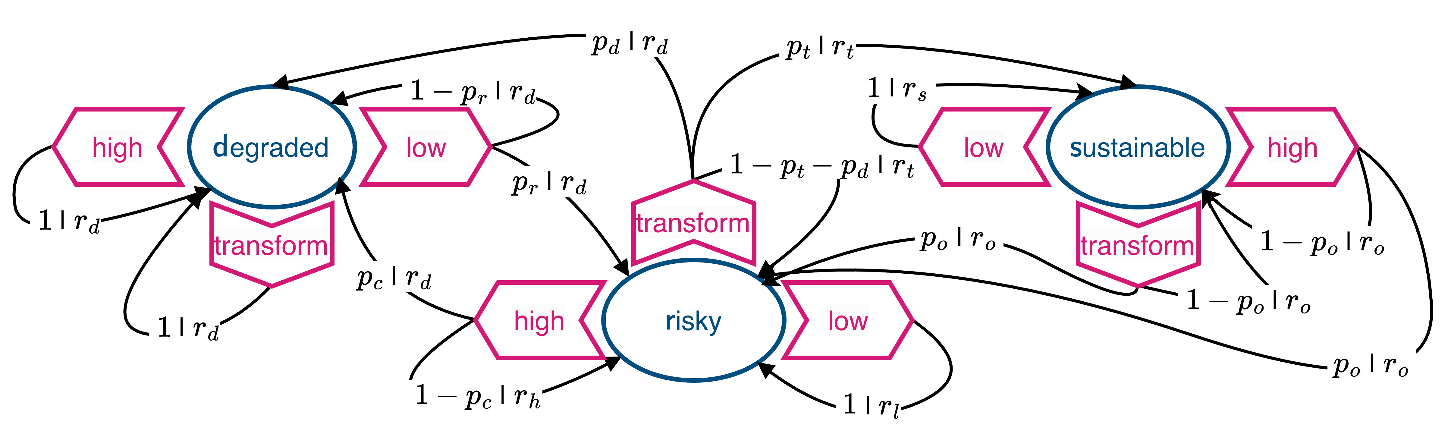
The low-intensity action at the risky state guarantees to stay in the risky environment but requires a reduction of immediate welfare (low-intensity reward \(r_l <\) high-intensity reward \(r_h\)).
High immediate welfare (\(r_h\)) via the high-intensity action at the risky state comes at the cost of over-using Nature, which may tip into a degraded state (with collapse probability \(p_c\)), where only a low-intensity course of action may recover Nature eventually (with recovery probability \(p_r\)).
Whenever the degraded state is involved, the agent only receives the lowest degradation reward \(r_d\).
An alternative to the cautious low-intensity action at the risky state is the transformation action, where eventually high levels of sustainable wellbeing \(r_s > r_h\) can be achieved (after the transition to the sustainable state with transition probability \(p_t\)).
However, the transition to the sustainable state requires investment into the transformation technology and thus lower immediate wellbeing during the transition (transition reward \(r_t < r_l\)).
It also may not guarantee to stay within the risky state and may cause Nature to degrade (with probability \(p_d\)).
Rebound effects. At the sustainable state, however, there is the risk of overusing the transformation technology (if another action than the low-intensity is taken) since this yields the highest overuse reward \(r_o\), which risks (with probability \(p_o\)) the relapse back into the risky environmental state.
Step 1 | Transition and rewards tensors
Transform the description of the MDP into two Python functions that can be called with the model parameters and return a transition and reward tensor, respectively. Make sure to write these functions to be used both with numpy and sympy.
# ...Test that both functions work and check that the transition tensors are proper probability distributions for three exemplary parameter combinations.
# ...Step 2 | State values
Write a Python function to numerically compute the MDP’s state values, given a policy_Xsa, a transitions_Tsas tensor, a rewards_Rsas tensor, and a discount factor dcf.
# ...Test that your function works with some arbitrary values for the policy_Xsa, transitions_Tsas tensor, rewards_Rsas tensors, and discount factor dcf.
# ...Step 3 | Policies
Formulate four different policies and represent them in Python:
The cautious policy always chooses the low-intensity action.
# ...The risky policy chooses the high-intensity action in the risky and sustainable state and the low-intensity action in the degraded state.
# ...The transformation policy chooses the transformation action in the risky state and the low-intensity action in the sustainable and degraded state.
# ...The overuse policy chooses the transformation action in the risky and sustainable state and the low-intensity action in the degraded state.
# ...Step 4 | Optimal policy
What are the state values of the risky state for all the four policies at the parameter combination \(p_c=0.2\), \(p_r=0.01\), \(p_t=0.04\), \(p_d=0.005\), \(p_o=0.02\), \(\gamma=0.98\), \(r_o=1.2\), \(r_s=1.0\), \(r_h=0.9\), \(r_l=0.7\), \(r_t=0.65\), \(r_d=0.0\)?
pc = 0.2; pr = 0.01; pt = 0.04; pd = 0.005; po = 0.02;
ro = 1.2; rs = 1.0; rh = 0.9; rl = 0.7; rt = 0.65; rd = 0.0
# ...Which is, therefore, the optimal policy for that parameter combination?
# ...Step 5 | Optimal policies with uncertainty
Given the other above parameters, how does the optimal policy change with a varying discount factor \(\gamma\)? Create a plot that shows the state values of the risky state for the four policies at \(\gamma \in [0.001, 0.9999]\) and interpret your result.
# ...